【从零构建大模型】二、编码Attention机制

概览

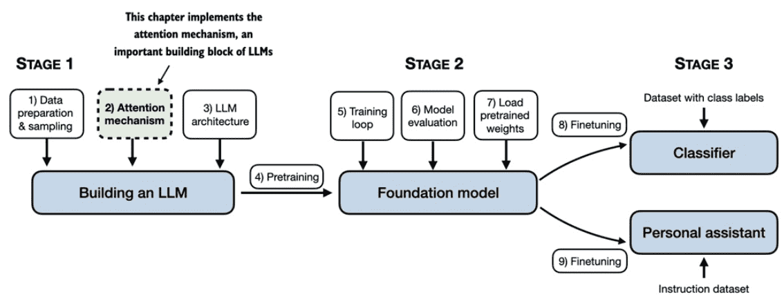
构建大模型的全景图如下,本文介绍了基础的attention处理。
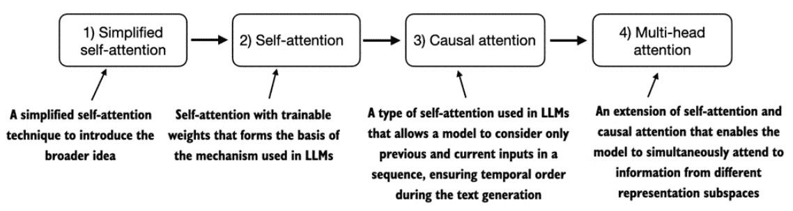
介绍的脉络如下:

介绍

The problem with modeling long sequences

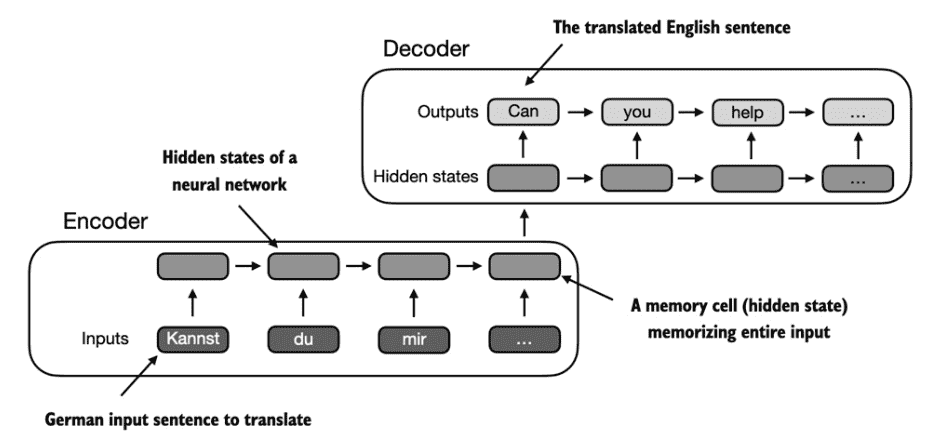
对于类似翻译的任务,由于不同语言的语法问题,所以难以做到一对一的逐字翻译,需要提前对原本的字符串进行encoder提取信息,然后使用decoder模块进行翻译。

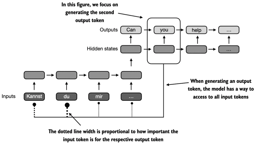
而传统的encoder-decoder RNNs方法在encoder阶段无法从编码器访问先前的隐藏状态。因此,它只能依赖于当前隐藏状态,而当前隐藏状态包含了所有相关信息。这可能会导致上下文丢失,尤其是在依赖关系可能跨越很长距离的复杂句子中。

所以提出了注意力机制来更好地捕获原本的信息。

Capturing data dependencies with attention mechanisms

在注意力机制中,encoder可以选择性地访问所有输入的tokens,并自行判断哪些tokens更加重要,而这部分判断就是依靠attention weights

Self attention是transfomer中的关键的一种机制,它允许输入序列中的每个位置在计算序列的表示时关注同一序列中的所有位置。自注意力机制是基于 Transformer 架构的当代LLM的关键组成部分,例如 GPT 系列。下面我们将从头开始编写这种自注意力机制的代码

Attending to different parts of the input with self-attention

A simple self-attention mechanism without trainable weights

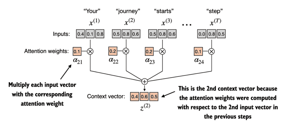
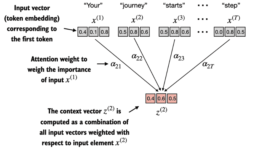
自注意力机制的目标是为每个输入元素计算一个上下文向量,该向量结合了所有其他输入元素的信息。

下图表示了一种简化后的attention机制,我们想要计算得到第2个字符的上下文向量就只需要用attention weights与原序列中的各个token相乘即可。

而一个简单的计算两者attention weights的方法就是直接将两者的token embedding进行点积。

点积还是相似性的度量,因为它量化了两个向量的对齐程度:更高的点积表示更大程度的对齐或相似性向量之间。在自注意力机制的背景下,点积决定了序列中元素相互关注的程度:点积越高,两个元素之间的相似度和注意力分数就越高。

通过点积得到attention weights后往往还会进行归一化,一般采用softmax函数。

最后通过各个token的embeddings与attention weights的加权相乘就可以得到需要的上下文向量。

简单的代码实现如下

1
2
3
4
5
6
7
8
9
10
11
12
13
14
15
16
17
18
19
20
21
22
23
24
25
26
27
28
29
30
31
32
33
34
import torch

inputs = torch.tensor(
[[0.43, 0.15, 0.89], # Your (x^1)
[0.55, 0.87, 0.66], # journey (x^2)
[0.57, 0.85, 0.64], # starts (x^3)
[0.22, 0.58, 0.33], # with (x^4)
[0.77, 0.25, 0.10], # one (x^5)
[0.05, 0.80, 0.55]] # step (x^6)
)

query = inputs[1] # 2nd input token is the query

attn_scores_2 = torch.empty(inputs.shape[0])
for i, x_i in enumerate(inputs):
attn_scores_2[i] = torch.dot(x_i, query) # dot product (transpose not necessary here since they are 1-dim vectors)

print(attn_scores_2)

def softmax_naive(x):
return torch.exp(x) / torch.exp(x).sum(dim=0)

attn_weights_2_naive = softmax_naive(attn_scores_2)

print("Attention weights:", attn_weights_2_naive)
print("Sum:", attn_weights_2_naive.sum())

query = inputs[1] # 2nd input token is the query

context_vec_2 = torch.zeros(query.shape)
for i,x_i in enumerate(inputs):
context_vec_2 += attn_weights_2[i]*x_i

print(context_vec_2)

Computing attention weights for all input tokens

前面说的是单个token如何计算上下文向量, 而在实际过程中可以简单的使用向量处理的方向一次性得到所有的attention weight和上下文向量,代码如下:

1
2
3
4
5
6
7
8
attn_scores = inputs @ inputs.T
print(attn_scores)

attn_weights = torch.softmax(attn_scores, dim=-1)
print(attn_weights)

all_context_vecs = attn_weights @ inputs
print(all_context_vecs)

Implementing self-attention with trainable weights

Computing the attention weights step by step

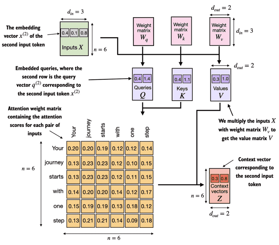
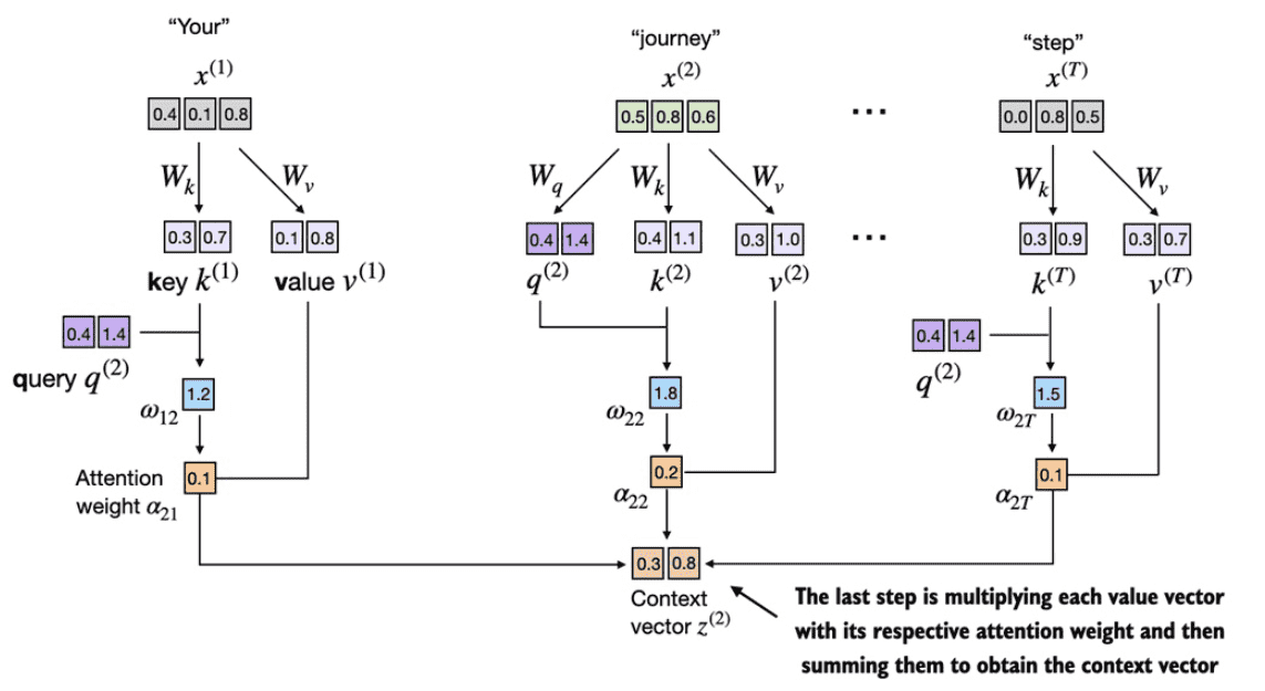
在实际的self-attention中会三个可训练的权重矩阵$$W_q$$,$$W_k$$,$$W_v$$,其分别用于与原token embedding相乘计算Query、Key、Value。下面以d_in=3维度的token以及d_out=2维度的输出来演示如何计算第二token的上下文。

请注意,在类似 GPT 的模型中,输入和输出维度通常相同,但为了便于说明,为了更好地跟踪计算,我们在此选择不同的输入(d_in=3)和输出(d_out=2)维度。

整体流程如下图所示:

  1. 各个token与$$W_q$$,$$W_k$$,$$W_v$$相乘的到q、k、v

  2. 第二个token的q与各个k相乘的到attention

  3. 对attention进行softmax

  4. 对attention进行缩放

  5. 各个attention与v加权相乘得到上下文向量

为什么在自注意力机制中会用嵌入维度的平方根来缩放点积?

  • 缩放的目的:用嵌入维度的平方根来缩放,是为了避免训练过程中出现过小的梯度。若不做缩放,训练时可能会遇到梯度非常小的情况,导致模型学习变慢,甚至陷入停滞。

  • 出现梯度变小的原因:1、当嵌入维度(即向量的维度)增加时,两个向量的点积值会变大。在GPT等大型语言模型(LLM)中,嵌入维度往往很高,可能达到上千,因此点积也变得很大。 2、在点积结果上应用softmax 函数时,如果数值较大,softmax 输出的概率分布会变得很尖锐,近似于阶跃函数。此时,大部分概率集中在几个值上,导致其他部分的梯度几乎为零。这样就会导致模型训练时更新不充分。

  • 缩放的效果:通过用嵌入维度的平方根缩放点积的大小,可以让点积的数值控制在合理范围,使得softmax 函数的输出更加平滑,从而使得梯度较大,模型可以更有效地学习。这种缩放的自注意力机制因此被称为“缩放点积注意力” (scaled-dot product attention)。

整体的代码如下所示:

1
2
3
4
5
6
7
8
9
10
11
12
13
14
15
16
17
18
19
20
21
22
23
24
25
26
27
28
29
30
31
32
33
34
35
36
37
38
39
40
41
42
43
44
45
46
47
import torch
inputs = torch.tensor(
[[0.43, 0.15, 0.89], # Your (x^1)
[0.55, 0.87, 0.66], # journey (x^2)
[0.57, 0.85, 0.64], # starts (x^3)
[0.22, 0.58, 0.33], # with (x^4)
[0.77, 0.25, 0.10], # one (x^5)
[0.05, 0.80, 0.55]] # step (x^6)
)

x_2 = inputs[1] #A
d_in = inputs.shape[1] #B = 3
d_out = 2 #C

# Initialize the three weight matrices Wq, Wk, and Wv
torch.manual_seed(123)
W_query = torch.nn.Parameter(torch.rand(d_in, d_out), requires_grad=False)
W_key = torch.nn.Parameter(torch.rand(d_in, d_out), requires_grad=False)
W_value = torch.nn.Parameter(torch.rand(d_in, d_out), requires_grad=False)
# 示例结构: shape=(3,2)
# tensor([[0.3821, 0.6605],
# [0.8536, 0.5932],
# [0.6367, 0.9826]])
# 说明
# setting requires_grad=False to reduce clutter in the outputs for illustration purposes
# 正式使用时需要设置 requires_grad=True

query_2 = x_2 @ W_query

# 虽然这儿只计算context vector`Z^(2)`,但仍然需要所有输入元素的键和值向量
# obtain all keys and values via matrix multiplication
keys = inputs @ W_key
values = inputs @ W_value
print("keys.shape:", keys.shape)
# 输出
# keys.shape: torch.Size([6, 2])

attn_scores_2 = query_2 @ keys.T
# All attention scores for given queryprint(attn_scores_2)
# 输出
# tensor([1.2705, 1.8524, 1.8111, 1.0795, 0.5577, 1.5440])

d_k = keys.shape[-1]attn_weights_2 = torch.softmax(attn_scores_2 / d_k**0.5, dim=-1)print(attn_weights_2)

# 输出
# tensor([0.1500, 0.2264, 0.2199, 0.1311, 0.0906, 0.1820])
context_vec_2 = attn_weights_2 @ valuesprint(context_vec_2)# 输出# tensor([0.3061, 0.8210])

Implementing a compact SelfAttention class

类似的在实际计算所有的上下文向量的时候都是通过矩阵相乘的方法来做的,如下图所示:

代码如下所示,注意这里使用了nn.Linear,这有助于更稳定、有效的模型训练。:

1
2
3
4
5
6
7
8
9
10
11
12
13
14
15
16
17
18
19
20
21
22
23
24
25
26
27
28
29
class SelfAttention_v2(nn.Module):
def __init__(self, d_in, d_out, qkv_bias=False):
super().__init__()
self.d_out = d_out
self.W_query = nn.Linear(d_in, d_out, bias=qkv_bias)
self.W_key = nn.Linear(d_in, d_out, bias=qkv_bias)
self.W_value = nn.Linear(d_in, d_out, bias=qkv_bias)
def forward(self, x):
keys = self.W_key(x)
queries = self.W_query(x)
values = self.W_value(x)

attn_scores = queries @ keys.T

attn_weights = torch.softmax(attn_scores / keys.shape[-1]**0.5, dim)

context_vec = attn_weights @ values
return context_vec

torch.manual_seed(789)
sa_v2 = SelfAttention_v2(d_in, d_out)
print(sa_v2(inputs))
# 输出
tensor([[-0.0739, 0.0713],
[-0.0748, 0.0703],
[-0.0749, 0.0702],
[-0.0760, 0.0685],
[-0.0763, 0.0679],
[-0.0754, 0.0693]], grad_fn=<MmBackward0>)

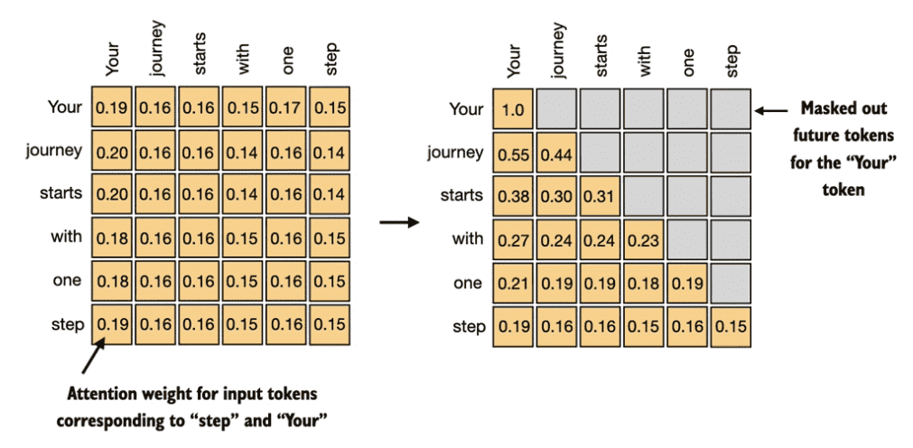
Hiding future words with causal attention

在decoder生成阶段时我们只能看到要生成的token的前面的token,所以需要对生成的attention weight进行mask,这也叫做Causal attention。

Applying a causal attention mask

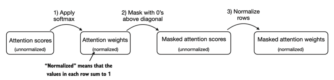
简单的mask就是在生成了attention weight之后在进行mask,然后再进行归一化。

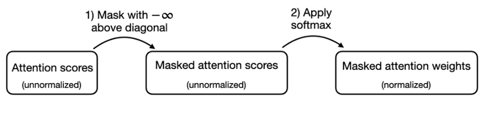
而更常见的方法是利用softmax的数学特性,在q@k得到attention之后直接给要mask的attention weights记为-inf,这样softmax之后其值为0。

代码实现如下:

1
2
3
4
5
6
7
8
9
10
11
12
13
14
15
16
17
18
19
20
21
22
23
mask = torch.triu(torch.ones(context_length, context_length), diagonal=1)
masked = attn_scores.masked_fill(mask.bool(), -torch.inf)
print(masked)
# 输出
tensor([[0.2899, -inf, -inf, -inf, -inf, -inf],
[0.4656, 0.1723, -inf, -inf, -inf, -inf],
[0.4594, 0.1703, 0.1731, -inf, -inf,
[0.2642, 0.1024, 0.1036, 0.0186, -inf,
[0.2183, 0.0874, 0.0882, 0.0177, 0.0786,
[0.3408, 0.1270, 0.1290, 0.0198, 0.1290, 0.0078]],
grad_fn=<MaskedFillBackward0>)


attn_weights = torch.softmax(masked / keys.shape[-1]**0.5, dim=1)
print(attn_weights)
# 输出(已经规范化,不用再额外操作了,节省了操作)
tensor([[1.0000, 0.0000, 0.0000, 0.0000, 0.0000, 0.0000],
[0.5517, 0.4483, 0.0000, 0.0000, 0.0000, 0.0000],
[0.3800, 0.3097, 0.3103, 0.0000, 0.0000, 0.0000],
[0.2758, 0.2460, 0.2462, 0.2319, 0.0000, 0.0000],
[0.2175, 0.1983, 0.1984, 0.1888, 0.1971, 0.0000],
[0.1935, 0.1663, 0.1666, 0.1542, 0.1666, 0.1529]],
grad_fn=<SoftmaxBackward0>)

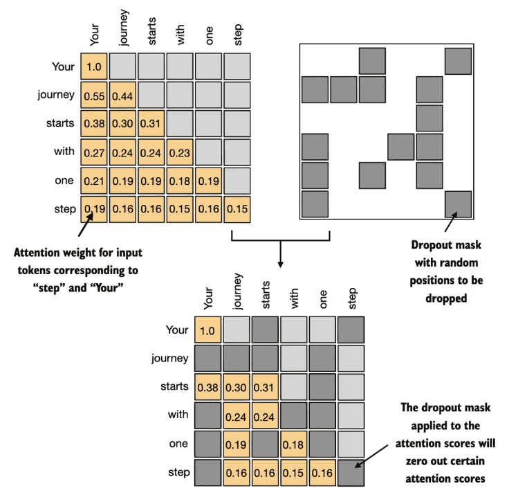
Masking additional attention weights with dropout

此外,我们还应用dropout来减少训练过程中的过拟合,确保模型不会过度依赖任何特定的隐藏层单元集。需要强调的是,Dropout 仅在训练期间使用,训练结束后将被禁用。

可以有两处dropout的地方

  1. 在计算完attention weight之后

  2. 在attention weight与values相乘之后

一般第一种更加普遍,下图我们以50%的dropout 比例为例来介绍,在实际如GPT模型中往往只会采取10%、20%的比例。

代码如下:

1
2
3
4
5
6
7
8
9
10
11
torch.manual_seed(123)
dropout = torch.nn.Dropout(0.5) #A
example = torch.ones(6, 6) #B
print(dropout(example))
# 输出(有近一半是0)
tensor([[2., 2., 0., 2., 2., 0.],
[0., 0., 0., 2., 0., 2.],
[2., 2., 2., 2., 0., 2.],
[0., 2., 2., 0., 0., 2.],
[0., 2., 0., 2., 0., 2.],
[0., 2., 2., 2., 2., 0.]])

Implementing a compact causal self-attention class

将mask和dropout的特性加上后的代码如下:

1
2
3
4
5
6
7
8
9
10
11
12
13
14
15
16
17
18
19
20
21
22
23
24
25
26
27
28
29
30
31
32
33
34
35
36
37
38
39
40
41
42
43
44
45
46
47
48
49
50
51
52
53
class CausalAttention(nn.Module):

def __init__(self, d_in, d_out, context_length,
dropout, qkv_bias=False):
super().__init__()
self.d_out = d_out
self.W_query = nn.Linear(d_in, d_out, bias=qkv_bias)
self.W_key = nn.Linear(d_in, d_out, bias=qkv_bias)
self.W_value = nn.Linear(d_in, d_out, bias=qkv_bias)
self.dropout = nn.Dropout(dropout) # A
self.register_buffer(
'mask',
torch.triu(
torch.ones(context_length, context_length),
diagonal=1
)
) #B


def forward(self, x):
b, num_tokens, d_in = x.shape #C
keys = self.W_key(x)
queries = self.W_query(x)
values = self.W_value(x)

attn_scores = queries @ keys.transpose(1, 2) #C
attn_scores.masked_fill_( #D
self.mask.bool()[:num_tokens, :num_tokens], -torch.inf)
attn_weights = torch.softmax(attn_scores / keys.shape[-1]**0.5, dim=-1)
attn_weights = self.dropout(attn_weights)

context_vec = attn_weights @ values
return context_vec


import torch
inputs = torch.tensor(
[[0.43, 0.15, 0.89], # Your (x^1)
[0.55, 0.87, 0.66], # journey (x^2)
[0.57, 0.85, 0.64], # starts (x^3)
[0.22, 0.58, 0.33], # with (x^4)
[0.77, 0.25, 0.10], # one (x^5)
[0.05, 0.80, 0.55]] # step (x^6)
)
batch = torch.stack((inputs, inputs), dim=0)

torch.manual_seed(123)
context_length = batch.shape[1]
ca = CausalAttention(d_in, d_out, context_length, 0.0)
context_vecs = ca(batch)
print("context_vecs.shape:", context_vecs.shape)
# 输出
# context_vecs.shape: torch.Size([2, 6, 2])

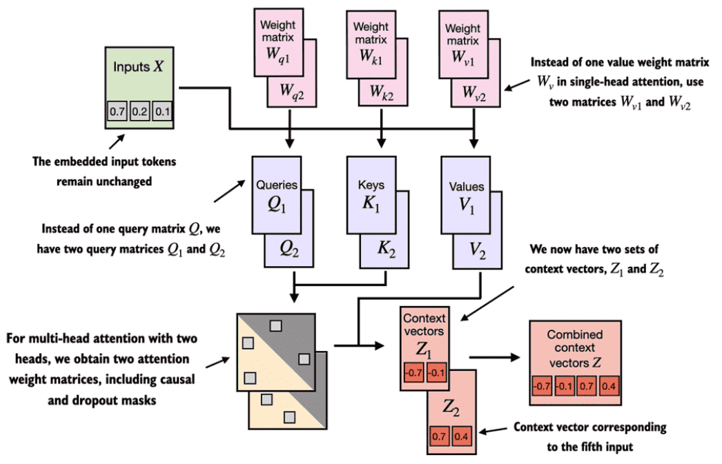
Extending single-head attention to multi-head attention

Stacking multiple single-head attention layers

实际往往会采取多头注意力机制,在分别得到对应的上下文后会将其直接进行拼接,然后一般会再与一个全联接层进行相乘

简单地将上述的代码进行包装就可以得到多头注意力的版本:

1
2
3
4
5
6
7
8
9
10
11
12
13
14
15
16
17
18
19
20
21
22
23
24
25
26
27
28
29
30
31
32
33
34
35
36
37
38
39
40
41
class MultiHeadAttentionWrapper(nn.Module):

def __init__(self, d_in, d_out, context_length, dropout, num_heads, qkv_bias=False):
super().__init__()
self.heads = nn.ModuleList(
[CausalAttention(d_in, d_out, context_length, dropout, qkv_bias)
for _ in range(num_heads)]
)

def forward(self, x):
return torch.cat([head(x) for head in self.heads], dim=-1)


torch.manual_seed(123)

context_length = batch.shape[1] # This is the number of tokens
d_in, d_out = 3, 2
mha = MultiHeadAttentionWrapper(
d_in, d_out, context_length, 0.0, num_heads=2
)

context_vecs = mha(batch)

print(context_vecs)
print("context_vecs.shape:", context_vecs.shape)

# 输出
tensor([[[-0.4519, 0.2216, 0.4772, 0.1063],
[-0.5874, 0.0058, 0.5891, 0.3257],
[-0.6300, -0.0632, 0.6202, 0.3860],
[-0.5675, -0.0843, 0.5478, 0.3589],
[-0.5526, -0.0981, 0.5321, 0.3428],
[-0.5299, -0.1081, 0.5077, 0.3493]],

[[-0.4519, 0.2216, 0.4772, 0.1063],
[-0.5874, 0.0058, 0.5891, 0.3257],
[-0.6300, -0.0632, 0.6202, 0.3860],
[-0.5675, -0.0843, 0.5478, 0.3589],
[-0.5526, -0.0981, 0.5321, 0.3428],
[-0.5299, -0.1081, 0.5077, 0.3493]]], grad_fn=<CatBackward0>)
context_vecs.shape: torch.Size([2, 6, 4])

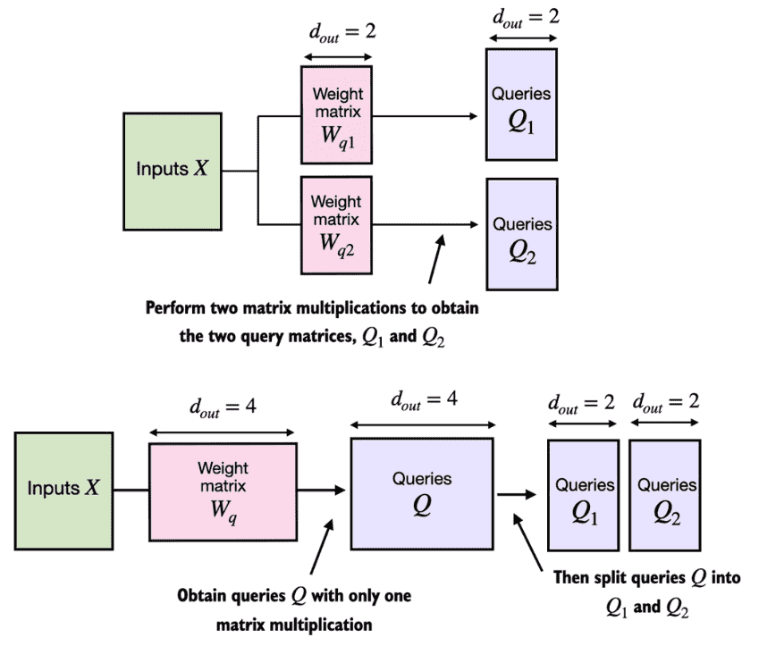
Implementing multi-head attention with weight splits

在实际的处理中,为了更好的并行化,其实会作为一个大矩阵来计算多头注意力。例如我们会一次性初始化一个大的Wq,然后通过一次矩阵运算得到Q后再对其进行形状的转化,分割成多个self-attention中的Q。再计算得到attention,再计算得到上下文,最后又通过形状的变化得到拼接后的输出。

1
2
3
4
5
6
7
8
9
10
11
12
13
14
15
16
17
18
19
20
21
22
23
24
25
26
27
28
29
30
31
32
33
34
35
36
37
38
39
40
41
42
43
44
45
46
47
48
49
50
51
52
53
54
55
56
57
58
59
60
61
62
63
64
65
66
67
68
69
70
71
72
73
74
75
76
77
78
79
80
81
82
83
84
85
86
87
88
89
90
91
92
class MultiHeadAttention(nn.Module):
def __init__(self, d_in, d_out, context_length, dropout, num_heads, qkv_bias=False):
super().__init__()
assert (d_out % num_heads == 0), \
"d_out must be divisible by num_heads"

self.d_out = d_out
self.num_heads = num_heads
self.head_dim = d_out // num_heads # Reduce the projection dim to match desired output dim

self.W_query = nn.Linear(d_in, d_out, bias=qkv_bias)
self.W_key = nn.Linear(d_in, d_out, bias=qkv_bias)
self.W_value = nn.Linear(d_in, d_out, bias=qkv_bias)
self.out_proj = nn.Linear(d_out, d_out) # Linear layer to combine head outputs
self.dropout = nn.Dropout(dropout)
self.register_buffer(
"mask",
torch.triu(torch.ones(context_length, context_length),
diagonal=1)
)

def forward(self, x):
b, num_tokens, d_in = x.shape
# As in `CausalAttention`, for inputs where `num_tokens` exceeds `context_length`,
# this will result in errors in the mask creation further below.
# In practice, this is not a problem since the LLM (chapters 4-7) ensures that inputs
# do not exceed `context_length` before reaching this forwar

keys = self.W_key(x) # Shape: (b, num_tokens, d_out)
queries = self.W_query(x)
values = self.W_value(x)

# We implicitly split the matrix by adding a `num_heads` dimension
# Unroll last dim: (b, num_tokens, d_out) -> (b, num_tokens, num_heads, head_dim)
keys = keys.view(b, num_tokens, self.num_heads, self.head_dim)
values = values.view(b, num_tokens, self.num_heads, self.head_dim)
queries = queries.view(b, num_tokens, self.num_heads, self.head_dim)

# Transpose: (b, num_tokens, num_heads, head_dim) -> (b, num_heads, num_tokens, head_dim)
keys = keys.transpose(1, 2)
queries = queries.transpose(1, 2)
values = values.transpose(1, 2)

# Compute scaled dot-product attention (aka self-attention) with a causal mask
# attn_scores Shape: (b, num_heads, num_tokens, num_tokens)
attn_scores = queries @ keys.transpose(2, 3) # Dot product for each head

# Original mask truncated to the number of tokens and converted to boolean
mask_bool = self.mask.bool()[:num_tokens, :num_tokens]

# Use the mask to fill attention scores
attn_scores.masked_fill_(mask_bool, -torch.inf)

attn_weights = torch.softmax(attn_scores / keys.shape[-1]**0.5, dim=-1)
attn_weights = self.dropout(attn_weights)

# (b, num_heads, num_tokens, num_tokens) @ (b, num_heads, num_tokens, head_dim) = (b, num_heads, num_tokens, head_dim)
# Shape: (b, num_tokens, num_heads, head_dim)
context_vec = (attn_weights @ values).transpose(1, 2)

# Combine heads, where self.d_out = self.num_heads * self.head_dim
context_vec = context_vec.contiguous().view(b, num_tokens, self.d_out)
context_vec = self.out_proj(context_vec) # optional projection

return context_vec

torch.manual_seed(123)

batch_size, context_length, d_in = batch.shape
d_out = 4
mha = MultiHeadAttention(d_in, d_out, context_length, 0.0, num_heads=2)

context_vecs = mha(batch)

print(context_vecs)
print("context_vecs.shape:", context_vecs.shape)

# 输出
tensor([[[ 0.1184, 0.3120, -0.0847, -0.5774],
[ 0.0178, 0.3221, -0.0763, -0.4225],
[-0.0147, 0.3259, -0.0734, -0.3721],
[-0.0116, 0.3138, -0.0708, -0.3624],
[-0.0117, 0.2973, -0.0698, -0.3543],
[-0.0132, 0.2990, -0.0689, -0.3490]],

[[ 0.1184, 0.3120, -0.0847, -0.5774],
[ 0.0178, 0.3221, -0.0763, -0.4225],
[-0.0147, 0.3259, -0.0734, -0.3721],
[-0.0116, 0.3138, -0.0708, -0.3624],
[-0.0117, 0.2973, -0.0698, -0.3543],
[-0.0132, 0.2990, -0.0689, -0.3490]]], grad_fn=<ViewBackward0>)
context_vecs.shape: torch.Size([2, 6, 4])

总结

  • 自注意力机制将上下文向量表示计算为输入的加权和。

  • 在简化的注意力机制中,注意力权重是通过点积计算的。

  • 在LLM中使用的自注意力机制(也称为缩放点积注意力机制)中,我们引入了可训练的权重矩阵来计算输入的中间变换:查询、值和键。当使用从左到右读取和生成文本的LLM时,我们添加了因果注意力掩码,以防止LLM访问未来的token。

  • 除了因果注意力掩码将注意力权重归零之外,我们还可以添加 dropout mask 来减少 LLM 中的过度拟合。

  • 基于 Transformer 的 LLM 中的注意力模块涉及因果注意力的多个实例,这称为多头注意力。

  • 我们可以通过堆叠多个因果注意模块实例来创建多头注意模块。

  • 创建多头注意力模块的更有效方法涉及分批矩阵乘法。

参考资料


【从零构建大模型】二、编码Attention机制
http://example.com/2025/05/02/LLMFromScratch2/
作者
滑滑蛋
发布于
2025年5月2日
许可协议