【从零构建大模型】三、从零实现一个 GPT 模型以生成文本

概览

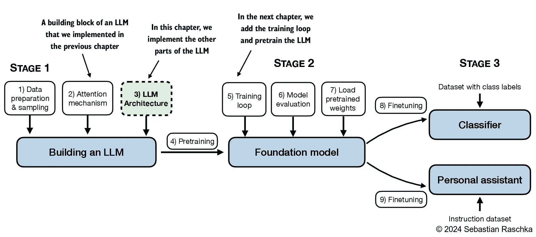
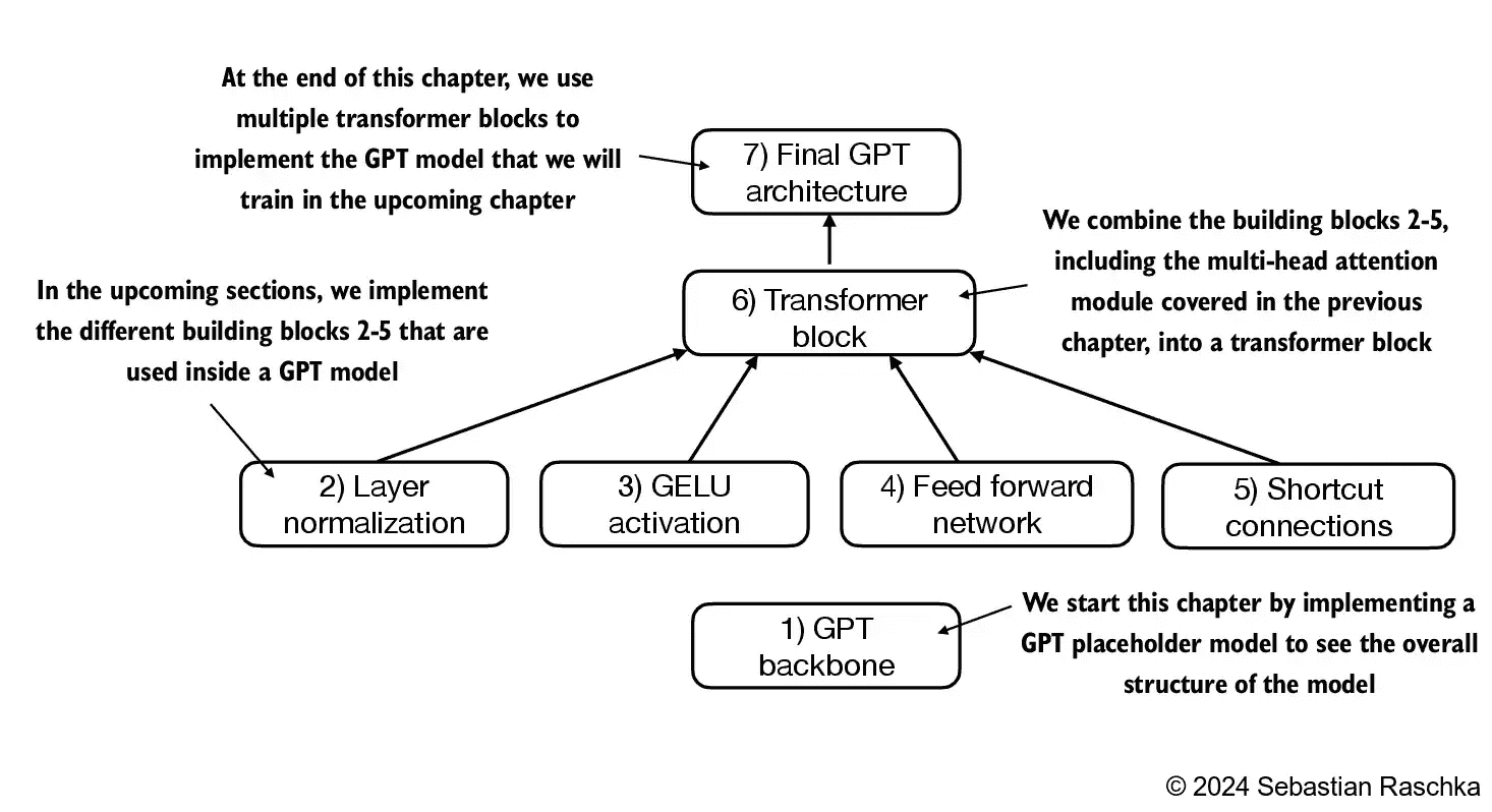
构建大模型的全景图如下，本文介绍了基础GPT-2系列的模型架构。

介绍的脉络如下：

介绍

Coding an LLM architecture

一个参数量为124 million的GPT-2模型包括了以下的定义参数：

GPT_CONFIG_124M = {
    "vocab_size": 50257,    # Vocabulary size
    "context_length": 1024, # Context length
    "emb_dim": 768,         # Embedding dimension
    "n_heads": 12,          # Number of attention heads
    "n_layers": 12,         # Number of layers
    "drop_rate": 0.1,       # Dropout rate
    "qkv_bias": False       # Query-Key-Value bias
}

vocab_size：单词数量，也就是BPE解码器所支持的单词数量
context_length：最长允许输入的token数量，也就是常说的上下文长度
emb_dim：Embedding层的维度
n_heads：多头注意力中注意力头的数量
n_layers：transformer块的数量
drop_rate：为了防止过拟合所采用的丢弃率，0.1意味着丢弃10%
qkv_bias：Liner层是否再加一个bias层

这些参数在初始化GPT模型的时候采用如下的使用方法（一些层还没有介绍，先留白）：

import torch
import torch.nn as nn


class DummyGPTModel(nn.Module):
    def __init__(self, cfg):
        super().__init__()
        self.tok_emb = nn.Embedding(cfg["vocab_size"], cfg["emb_dim"])
        self.pos_emb = nn.Embedding(cfg["context_length"], cfg["emb_dim"])
        self.drop_emb = nn.Dropout(cfg["drop_rate"])
        
        # Use a placeholder for TransformerBlock
        self.trf_blocks = nn.Sequential(
            *[DummyTransformerBlock(cfg) for _ in range(cfg["n_layers"])])
        
        # Use a placeholder for LayerNorm
        self.final_norm = DummyLayerNorm(cfg["emb_dim"])
        self.out_head = nn.Linear(
            cfg["emb_dim"], cfg["vocab_size"], bias=False
        )

    def forward(self, in_idx):
        batch_size, seq_len = in_idx.shape
        tok_embeds = self.tok_emb(in_idx)
        pos_embeds = self.pos_emb(torch.arange(seq_len, device=in_idx.device))
        x = tok_embeds + pos_embeds
        x = self.drop_emb(x)
        x = self.trf_blocks(x)
        x = self.final_norm(x)
        logits = self.out_head(x)
        return logits


class DummyTransformerBlock(nn.Module):
    def __init__(self, cfg):
        super().__init__()
        # A simple placeholder

    def forward(self, x):
        # This block does nothing and just returns its input.
        return x


class DummyLayerNorm(nn.Module):
    def __init__(self, normalized_shape, eps=1e-5):
        super().__init__()
        # The parameters here are just to mimic the LayerNorm interface.

    def forward(self, x):
        # This layer does nothing and just returns its input.
        return x

Normalizing activations with layer normalization

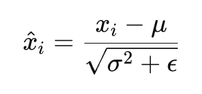
LayerNorm归一化层的作用是将某一个维度中的参数都均值化到0，同时将方差归为1。其处理方法如下：

$\mu = \frac{1}{N} \sum_{i=1}^{N} x_i$：均值
$\sigma^2 = \frac{1}{N} \sum_{i=1}^{N} (x_i - \mu)^2$：方差
$\varepsilon$：小值，防止除以0

而更灵活一点的实现会再额外添加了一个scale变量以控制各变量x进行缩放，还有shift变量来控制变量x进行平移。

简单使用代码实现，如下所示：

class LayerNorm(nn.Module):
    def __init__(self, emb_dim):
        super().__init__()
        self.eps = 1e-5
        self.scale = nn.Parameter(torch.ones(emb_dim))
        self.shift = nn.Parameter(torch.zeros(emb_dim))

    def forward(self, x):
        mean = x.mean(dim=-1, keepdim=True)
        var = x.var(dim=-1, keepdim=True, unbiased=False)
        norm_x = (x - mean) / torch.sqrt(var + self.eps)
        return self.scale * norm_x + self.shift

需要注意的是我们这里的x其实就是样本，所以 $\mu$实际上并不是标准的均值，故理论上在计算方差时应该除以N-1，不然就是有偏的。不过由于GPT-2的结构是这样的，所以我们仿照它的做法，此外由于embedding层的维数N一般都比较大，所以N和N-1也差别不大。

Implementing a feed forward network with GELU activations

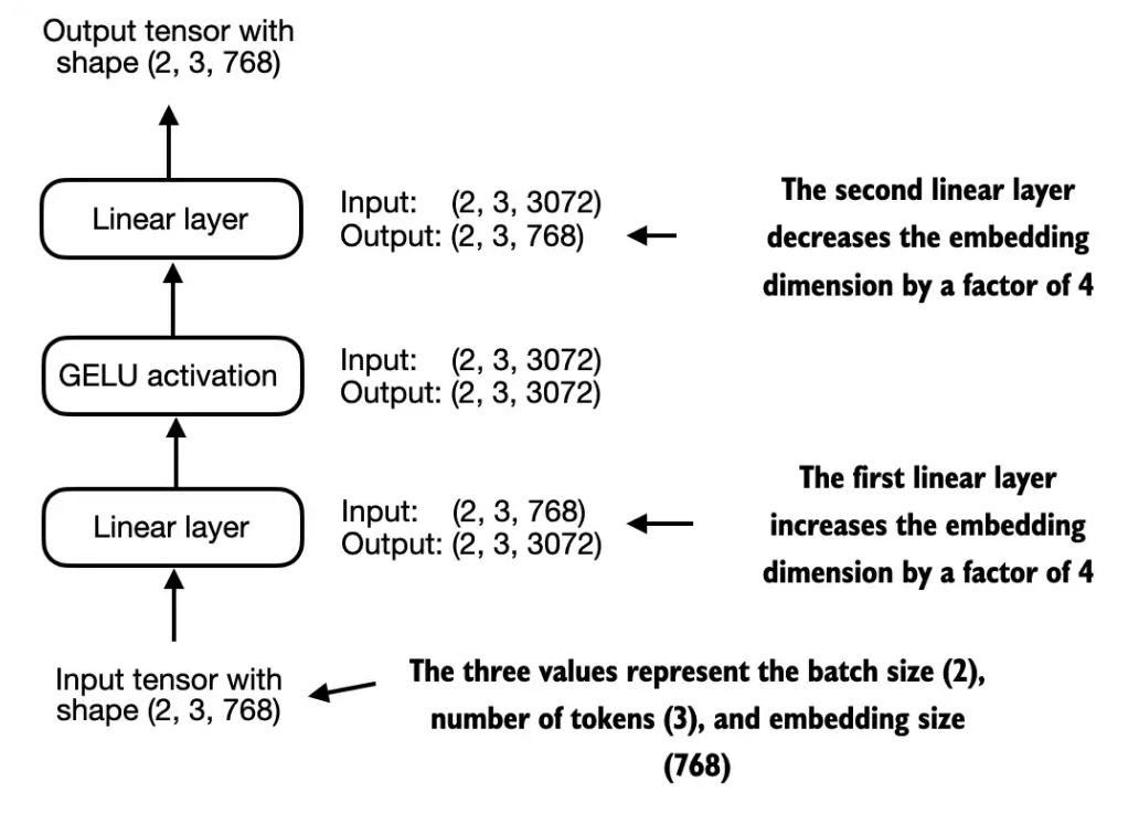
一个前馈网络的结构如下：

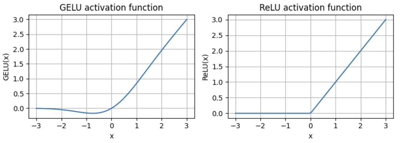
注意这里采用的是GELU激活函数，其表达式如下：

$$\text{GELU}(x) \approx 0.5 \cdot x \cdot \left(1 + \tanh\left[\sqrt{\frac{2}{\pi}} \cdot \left(x + 0.044715 \cdot x^3\right)\right]\right)$$

相比于RELU激活函数，GELU是一个平滑的非线性函数，近似于ReLU，但负值具有非零梯度（约-0.75除外）。

代码实现前馈网络如下：

class FeedForward(nn.Module):
    def __init__(self, cfg):
        super().__init__()
        self.layers = nn.Sequential(
            nn.Linear(cfg["emb_dim"], 4 * cfg["emb_dim"]),
            GELU(),
            nn.Linear(4 * cfg["emb_dim"], cfg["emb_dim"]),
        )

    def forward(self, x):
        return self.layers(x)

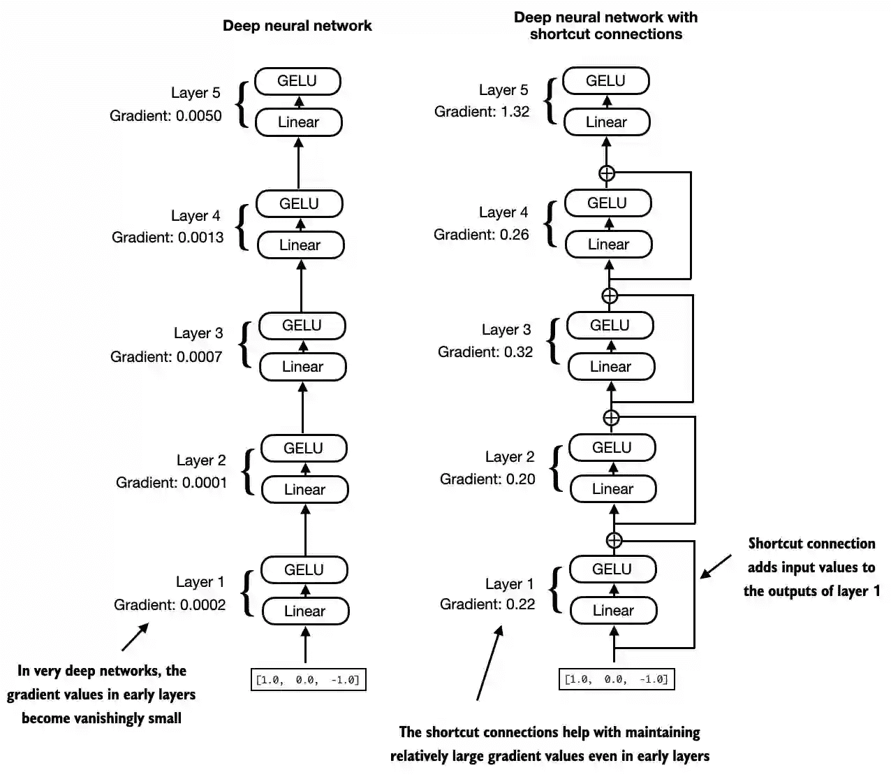
Adding shortcut connections

shortcut连接主要是为了解决梯度消息的问题，它将之前网络的输出与现在网络的输入相加后再进行传递，如下所示：

该机制的代码实现如下所示：

class ExampleDeepNeuralNetwork(nn.Module):
    def __init__(self, layer_sizes, use_shortcut):
        super().__init__()
        self.use_shortcut = use_shortcut
        self.layers = nn.ModuleList([
            nn.Sequential(nn.Linear(layer_sizes[0], layer_sizes[1]), GELU()),
            nn.Sequential(nn.Linear(layer_sizes[1], layer_sizes[2]), GELU()),
            nn.Sequential(nn.Linear(layer_sizes[2], layer_sizes[3]), GELU()),
            nn.Sequential(nn.Linear(layer_sizes[3], layer_sizes[4]), GELU()),
            nn.Sequential(nn.Linear(layer_sizes[4], layer_sizes[5]), GELU())
        ])

    def forward(self, x):
        for layer in self.layers:
            # Compute the output of the current layer
            layer_output = layer(x)
            # Check if shortcut can be applied
            if self.use_shortcut and x.shape == layer_output.shape:
                x = x + layer_output
            else:
                x = layer_output
        return x


def print_gradients(model, x):
    # Forward pass
    output = model(x)
    target = torch.tensor([[0.]])

    # Calculate loss based on how close the target
    # and output are
    loss = nn.MSELoss()
    loss = loss(output, target)
    
    # Backward pass to calculate the gradients
    loss.backward()

    for name, param in model.named_parameters():
        if 'weight' in name:
            # Print the mean absolute gradient of the weights
            print(f"{name} has gradient mean of {param.grad.abs().mean().item()}")
    
layer_sizes = [3, 3, 3, 3, 3, 1]  

sample_input = torch.tensor([[1., 0., -1.]])

torch.manual_seed(123)
model_without_shortcut = ExampleDeepNeuralNetwork(
    layer_sizes, use_shortcut=False
)
print_gradients(model_without_shortcut, sample_input)        

# 没有shortcut连接
# layers.0.0.weight has gradient mean of 0.00020173584925942123
# layers.1.0.weight has gradient mean of 0.00012011159560643137
# layers.2.0.weight has gradient mean of 0.0007152040489017963
# layers.3.0.weight has gradient mean of 0.0013988736318424344
# layers.4.0.weight has gradient mean of 0.005049645435065031

# 有shortcut连接
torch.manual_seed(123)
model_with_shortcut = ExampleDeepNeuralNetwork(
    layer_sizes, use_shortcut=True
)
print_gradients(model_with_shortcut, sample_input)
# layers.0.0.weight has gradient mean of 0.22169792652130127
# layers.1.0.weight has gradient mean of 0.20694108307361603
# layers.2.0.weight has gradient mean of 0.3289699852466583
# layers.3.0.weight has gradient mean of 0.2665732204914093
# layers.4.0.weight has gradient mean of 1.3258541822433472

Connecting attention and linear layers in a transformer block

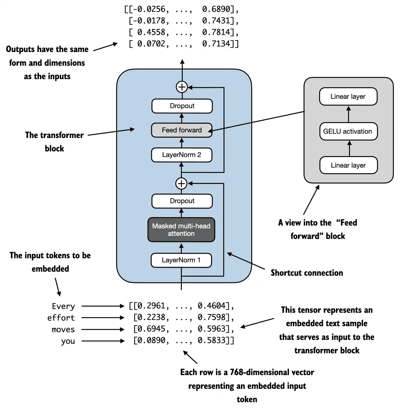
一个transformer块的结构如下所示：

简单的代码实现如下：

from previous_chapters import MultiHeadAttention

class TransformerBlock(nn.Module):
    def __init__(self, cfg):
        super().__init__()
        self.att = MultiHeadAttention(
            d_in=cfg["emb_dim"],
            d_out=cfg["emb_dim"],
            context_length=cfg["context_length"],
            num_heads=cfg["n_heads"], 
            dropout=cfg["drop_rate"],
            qkv_bias=cfg["qkv_bias"])
        self.ff = FeedForward(cfg)
        self.norm1 = LayerNorm(cfg["emb_dim"])
        self.norm2 = LayerNorm(cfg["emb_dim"])
        self.drop_shortcut = nn.Dropout(cfg["drop_rate"])

    def forward(self, x):
        # Shortcut connection for attention block
        shortcut = x
        x = self.norm1(x)
        x = self.att(x)  # Shape [batch_size, num_tokens, emb_size]
        x = self.drop_shortcut(x)
        x = x + shortcut  # Add the original input back

        # Shortcut connection for feed forward block
        shortcut = x
        x = self.norm2(x)
        x = self.ff(x)
        x = self.drop_shortcut(x)
        x = x + shortcut  # Add the original input back

        return x

transformer块采用这种结构的好处可以如下理解：

多头注意力机制可以识别并分析出序列中各元属之间的关系
前馈网络强化了局部的信息
对每个位置进行特定的非线性变换，提升其独立特征表达
协同效果：这种组合让模型既能捕捉全局模式，又能处理局部细节，从而在面对复杂数据模式时表现出更强的处理能力。
【例】句子翻译任务：自注意力机制帮助模型理解句子结构和词语之间的关系；前馈网络对每个单词的特定信息进行调整和优化，从而生成更准确的翻译。

注意对于整一个Transformer结构，其输入和输出的形状最后是相同的。这种输入输出相同的设计更加方便各层之间的叠加，输入可以直接当做输出叠加上去。

例如下面的这个示例，我们采用batch size=2，上下文长度为4，每个embedding层的维度为768，最后得到的结果也是相同的形状。

torch.manual_seed(123)

x = torch.rand(2, 4, 768)  # Shape: [batch_size, num_tokens, emb_dim]
block = TransformerBlock(GPT_CONFIG_124M)
output = block(x)

print("Input shape:", x.shape)
print("Output shape:", output.shape)

# Input shape: torch.Size([2, 4, 768])
# Output shape: torch.Size([2, 4, 768])

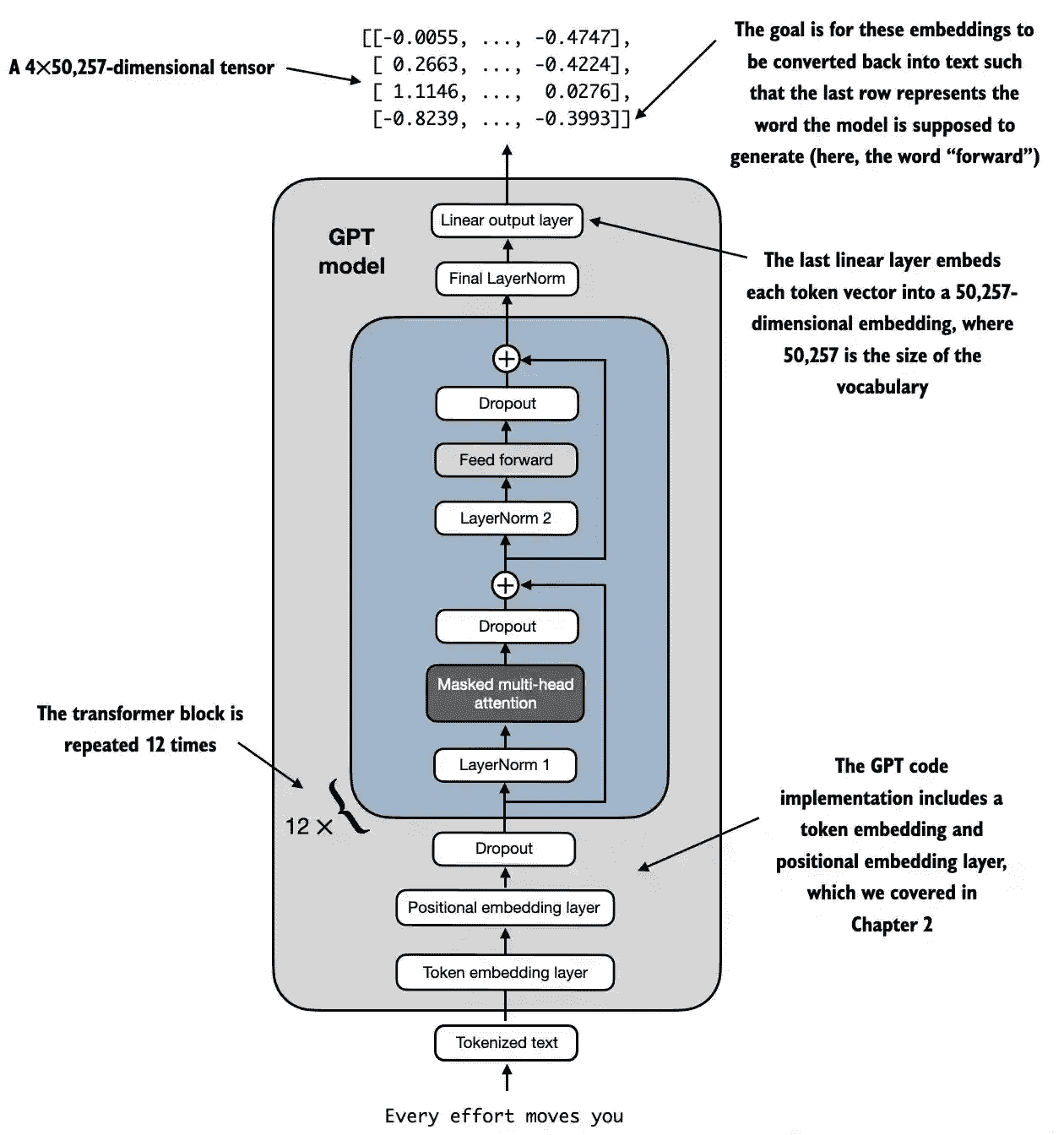
Coding the GPT model

一个GPT模型的结构概览如下图所示。

对于一个124 million参数的GPT-2模型，其使用了12个transformer块，对于最大的 GPT-2 模型，其参数有 1.542 billion，这个 Transformer 块重复了 36 次。

叠加起来的代码实现如下：

class GPTModel(nn.Module):
    def __init__(self, cfg):
        super().__init__()
        self.tok_emb = nn.Embedding(cfg["vocab_size"], cfg["emb_dim"])
        self.pos_emb = nn.Embedding(cfg["context_length"], cfg["emb_dim"])
        self.drop_emb = nn.Dropout(cfg["drop_rate"])

        self.trf_blocks = nn.Sequential(
            *[TransformerBlock(cfg) for _ in range(cfg["n_layers"])])

        self.final_norm = LayerNorm(cfg["emb_dim"])
        self.out_head = nn.Linear(
            cfg["emb_dim"], cfg["vocab_size"], bias=False
        )

    def forward(self, in_idx):
        batch_size, seq_len = in_idx.shape
        tok_embeds = self.tok_emb(in_idx)
        pos_embeds = self.pos_emb(torch.arange(seq_len, device=in_idx.device))
        x = tok_embeds + pos_embeds  # Shape [batch_size, num_tokens, emb_size]
        x = self.drop_emb(x)
        x = self.trf_blocks(x)
        x = self.final_norm(x)
        logits = self.out_head(x)
        return logits

注意模型最后的输出的结果是后续接着各个词的对应id的概率，其维度为字典的大小。注意其实际上生成了这个上下文中各个前缀生成的可能的词的结果。

torch.manual_seed(123)
model = GPTModel(GPT_CONFIG_124M)

out = model(batch)
print("Input batch:\n", batch)
print("\nOutput shape:", out.shape)
print(out)

# 输出
Input batch:
 tensor([[6109, 3626, 6100,  345],
        [6109, 1110, 6622,  257]])

Output shape: torch.Size([2, 4, 50257])
tensor([[[ 0.1381,  0.0077, -0.1963,  ..., -0.0222, -0.1060,  0.1717],
         [ 0.3865, -0.8408, -0.6564,  ..., -0.5163,  0.2369, -0.3357],
         [ 0.6989, -0.1829, -0.1631,  ...,  0.1472, -0.6504, -0.0056],
         [-0.4290,  0.1669, -0.1258,  ...,  1.1579,  0.5303, -0.5549]],

        [[ 0.1094, -0.2894, -0.1467,  ..., -0.0557,  0.2911, -0.2824],
         [ 0.0882, -0.3552, -0.3527,  ...,  1.2930,  0.0053,  0.1898],
         [ 0.6091,  0.4702, -0.4094,  ...,  0.7688,  0.3787, -0.1974],
         [-0.0612, -0.0737,  0.4751,  ...,  1.2463, -0.3834,  0.0609]]],
       grad_fn=<UnsafeViewBackward0>)

参数量分析

GPT2各个size的参数如下：

GPT2-small (the 124M configuration we already implemented):
- “emb_dim” = 768
- “n_layers” = 12
- “n_heads” = 12
GPT2-medium:
- “emb_dim” = 1024
- “n_layers” = 24
- “n_heads” = 16
GPT2-large:
- “emb_dim” = 1280
- “n_layers” = 36
- “n_heads” = 20
GPT2-XL:
- “emb_dim” = 1600
- “n_layers” = 48
- “n_heads” = 25

我们代码实现的是GPT2-small，但是如果我们直接将所有的参数量都统计出来会发现其值并不是124M，而是163M：

model = GPTModel(GPT_CONFIG_124M)
total_params = sum(p.numel() for p in model.parameters())
print(f"Total number of parameters: {total_params:,}")
# Total number of parameters: 163,009,536

这是由于在最初的GPT-2模型中使用了模型参数绑定，也就是self.out_head.weight = self.tok_emb.weight。因为tok_emb负责将id转化为对应的embedding，其行数是50257，列数是768维，而out_head负责将embedding再转为字典中词数量的维度，故可以复用。

减去out_head这一层的参数量后也可以看到确实就是124M的参数量

1
2
3

total_params_gpt2 =  total_params - sum(p.numel() for p in model.out_head.parameters())
print(f"Number of trainable parameters considering weight tying: {total_params_gpt2:,}")
# Number of trainable parameters considering weight tying: 124,412,160

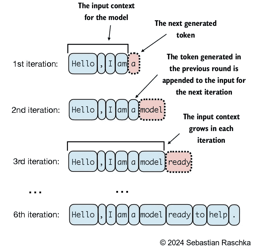
Generating text

下图展示了生成文本的一个经典过程，即每次生成一个新的token，然后再将这个token拼接起来继续生成后一个token。

一个简单的生成文本的代码实现如下所示，在这里我们将只取输出的n_token那一层的最后一维，代表利用前面全部的信息所得到的后一个词的预测结果，然后再简单地进行softmax选取概览最高的那一个词作为输出。

def generate_text_simple(model, idx, max_new_tokens, context_size):
    # idx is (batch, n_tokens) array of indices in the current context
    for _ in range(max_new_tokens):
        
        # Crop current context if it exceeds the supported context size
        # E.g., if LLM supports only 5 tokens, and the context size is 10
        # then only the last 5 tokens are used as context
        idx_cond = idx[:, -context_size:]
        
        # Get the predictions
        with torch.no_grad():
            logits = model(idx_cond)
        
        # Focus only on the last time step
        # (batch, n_tokens, vocab_size) becomes (batch, vocab_size)
        logits = logits[:, -1, :]  

        # Apply softmax to get probabilities
        probas = torch.softmax(logits, dim=-1)  # (batch, vocab_size)

        # Get the idx of the vocab entry with the highest probability value
        idx_next = torch.argmax(probas, dim=-1, keepdim=True)  # (batch, 1)

        # Append sampled index to the running sequence
        idx = torch.cat((idx, idx_next), dim=1)  # (batch, n_tokens+1)

    return idx

注意这时我们还没有对模型训练，所以模型前向传播得到的都是一些混乱的单词

start_context = "Hello, I am"

encoded = tokenizer.encode(start_context)
print("encoded:", encoded)
# encoded: [15496, 11, 314, 716]

encoded_tensor = torch.tensor(encoded).unsqueeze(0)
print("encoded_tensor.shape:", encoded_tensor.shape)
# encoded_tensor.shape: torch.Size([1, 4])

model.eval() # disable dropout

out = generate_text_simple(
    model=model,
    idx=encoded_tensor, 
    max_new_tokens=6, 
    context_size=GPT_CONFIG_124M["context_length"]
)

print("Output:", out)
print("Output length:", len(out[0]))
# Output: tensor([[15496,    11,   314,   716, 27018, 24086, 47843, 30961, 42348,  7267]])
# Output length: 10

decoded_text = tokenizer.decode(out.squeeze(0).tolist())
print(decoded_text)
# Hello, I am Featureiman Byeswickattribute argue

参考资料

https://knowledge.zhaoweiguo.com/build/html/x-learning/books/ais/2024/build\_llm\_from\_scratch#understanding-llm

LLM > 从零构建大模型

#大模型

【从零构建大模型】三、从零实现一个 GPT 模型以生成文本

http://example.com/2025/05/03/LLMFromScratch3/

作者

滑滑蛋

发布于

2025年5月3日

许可协议

【从零构建大模型】四、对模型进行无监督训练上一篇

【从零构建大模型】二、编码Attention机制下一篇