Afab并行
理论分析
最简单的pipeline并行就是将模型划分为好几层,然后分别放置在不同的GPU上依次进行前向传播和后先传播,如下图所示。但是这带来的最大的问题是效率过低,存在很多空闲时刻。
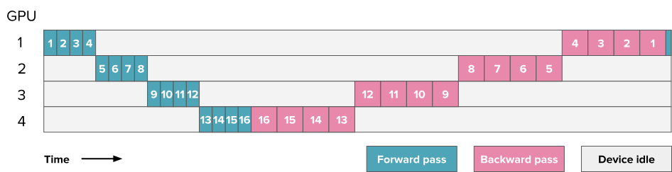
一个16层模型的流水线并行示例,该模型分布在4块GPU上。数字表示层编号。
假设$t_f$ 和$t_b$ 分别是单个微批次在流水线的一个阶段上进行前向传播和反向传播所需的时间(通常假设 $t_b\approx2\times t_f$,这在上图中可以观察到)。如果我们能够完美并行化,理想总时间应为 $t =t_b+t_f$。但由于流水线气泡的存在,额外的时间为$t_p =(p-1)*(t_b+t_f)$其中$p$ 是流水线并行度,即上图中的GPU数量),即每个GPU在其他GPU计算时的等待时间。
因此我们可以计算额外气泡时间与理想时间的比值:
$$r_{bubble}=\frac{(p-1)*(t_f+t_b)}{t_f+t_b}=p-1$$
当我们增加流水线阶段数时,气泡时间随之增加,GPU利用率下降。可以看出,在一个简单的实现中,流水线气泡可能会非常大!
为此需要提出一些优化方法来减少流水线中的气泡。一个经典的方法就是全前向-全反向(AFAB, All-Forward-All-Backward)调度。其整体思路是与微批次(microbatches)相绑定的。在微批次中,我们需要先对微批次中的所有的样本进行前向传播和反向传播,得到梯度后对各样本的梯度进行平均,然后通过优化器更新参数。
其优势在于前向和反向传播仍然是严格顺序的,因此可以保持模型训练代码的整体组织,使这种流水线并行实现方式成为最容易实现的一种。
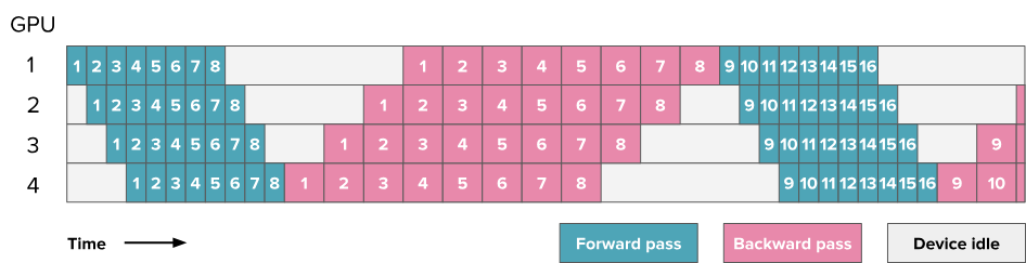
在之前的图表中,数字代表的是模型的层数,而从这一张图开始,所有流水线并行相关的图表中的数字都表示微批次。你可以将每个方块理解为包含多个层,就像前一张图所示的那样。
在如此设计下,理想情况下处理m个批次所需要的时间为 $t_{id}=m \times (t_f + t_b)$,实际过程中产生的气泡依旧为$(p-1)*(t_b+t_f)$,所以气泡比例为:
$$r_{bubble}=\frac{(p-1)*(t_f+t_b)}{m\times ({t_f+t_b})}=p-1$$
可以看到我们可以通过增加微批次的方法来减少气泡。
代码实现
1. pipeline_communicate
实现了流水线并行中各个阶段之间点对点的发送和接收张量(激活值或梯度)的通用接口。
1
2
3
4
5
6
7
8
9
10
11
12
13
14
15
16
17
18
19
20
21
22
23
24
25
26
27
28
29
30
31
32
33
34
35
36
37
38
39
40
41
42
43
44
45
46
47
48
49
50
51
52
53
54
55
56
57
58
59
60
61
62
63
64
65
|
STEP, VERBOSE = 0, os.environ.get("VERBOSE", "0") == "1"
def pipeline_communicate(operation, device, dtype, tensor=None, shapes=None):
"""
处理流水线阶段之间用于前向和反向传播的点对点通信。
Args:
operation (str): 通信操作的类型 ('recv_forward', 'send_forward',
'recv_backward', 'send_backward')
device: 张量操作的目标设备 (例如, CPU, GPU)
dtype: 张量的数据类型
tensor: 用于发送操作的输入张量 (默认: None)
shapes: 用于接收张量的形状规格 (默认: None)
Returns:
torch.Tensor or None: 接收操作返回接收到的张量,发送操作返回 None
"""
global STEP
global VERBOSE
if operation == 'recv_forward':
if pgm.process_group_manager.pp_is_first_stage: return None
tensor = torch.empty(shapes, requires_grad=True, device=device, dtype=dtype)
src = pgm.process_group_manager.pp_prev_rank
elif operation == 'send_forward':
if pgm.process_group_manager.pp_is_last_stage: return
dest = pgm.process_group_manager.pp_next_rank
elif operation == 'recv_backward':
if pgm.process_group_manager.pp_is_last_stage: return None
tensor = torch.empty(shapes, requires_grad=True, device=device, dtype=dtype)
src = pgm.process_group_manager.pp_next_rank
elif operation == 'send_backward':
if pgm.process_group_manager.pp_is_first_stage: return
dest = pgm.process_group_manager.pp_prev_rank
is_send = operation.startswith('send')
peer_rank = dest if is_send else src
op = dist.P2POp(dist.isend if is_send else dist.irecv, tensor, peer_rank)
if VERBOSE:
print(f"{operation} | {'sending' if is_send else 'receiving'} {operation.split('_')[1]} "
f"{pgm.process_group_manager.pp_rank} {'→' if is_send else '←'} {peer_rank} | "
f"STEP:{STEP} | RANK:{pgm.process_group_manager.pp_rank}", flush=True)
[req.wait() for req in dist.batch_isend_irecv([op])]
torch.cuda.synchronize()
if VERBOSE: STEP += 1
return tensor if not is_send else None
|
2. PipelineParallel
在初始化时,会将decoder_layers进行划分,根据pp分离的数量得到每个gpu负责多少layers,然后得到每个gpu负责的layer的起始与结束的decoder layer。还会看当前进程是否是pipeline的第一个进程,如果是就包含embedding层,不然就使用nn.Identity()。nn.Identity()的作用是将输入原封不动地返回。还会看如果当前进程时pipeline的最后一个进程,那么就会加上final_norm和final_proj,不然也是用nn.Identity()代替。
在forward的时候,其输入有input、position_ids和hidden_states。如果hidden_states不为空,那么输入就是input_ids,不然输入就是hidden_states,然后对输入使用embedding,因为如果不是第一个pipeline,embedding都是nn.Identity(),所以是可以的。然后执行自己所属的decoder_layers,然后在执行final_norma和final_proj。
在backward的时候,输入是input_tensor(当前阶段输入的tensor)、output_tensor(当前阶段输出的tensor)和output_tensor_grad(关于output_tensor的梯度)
首先需要设置input_tensor需要保存梯度,需要额外设置的原因在于原本非叶子结点是不保存的梯度的,但是现在模型进行了拆分,所以也需要保存。
然后需要查看output_tensor_grad是不是None,如果是None那就说明现在其实是在最后一个阶段,那就需要将其初始化为1
然后执行反向传播计算当前阶段的梯度。
然后如果不是第一个阶段,就继续往前传递梯度。
1
2
3
4
5
6
7
8
9
10
11
12
13
14
15
16
17
18
19
20
21
22
23
24
25
26
27
28
29
30
31
32
33
34
35
36
37
38
39
40
41
42
43
44
45
46
47
48
49
50
51
52
53
|
class PipelineParallel(nn.Module):
def __init__(self, model, config):
super().__init__()
layer_distribution = self.distribute_layers(config.num_hidden_layers)
self.embedding = model.embedding if pgm.process_group_manager.pp_is_first_stage else nn.Identity()
self.decoder_layers = nn.ModuleDict({str(i): model.decoder_layers[i] for i in layer_distribution})
self.final_norm = model.final_norm if pgm.process_group_manager.pp_is_last_stage else nn.Identity()
self.final_proj = model.final_proj if pgm.process_group_manager.pp_is_last_stage else nn.Identity()
def distribute_layers(self, num_layers):
"""计算当前流水线阶段应该负责哪些层。"""
layers_per_gpu = [num_layers // pgm.process_group_manager.pp_world_size + (1 if i < num_layers % pgm.process_group_manager.pp_world_size else 0) for i in range(pgm.process_group_manager.pp_world_size)]
start_layer = sum(layers_per_gpu[:pgm.process_group_manager.pp_rank])
return list(range(start_layer, start_layer + layers_per_gpu[pgm.process_group_manager.pp_rank]))
def forward(self, input_ids, position_ids, hidden_states):
"""当前流水线阶段的前向传播。"""
x = hidden_states if hidden_states is not None else input_ids
x = self.embedding(x)
for layer in self.decoder_layers.values():
x = layer(x, position_ids=position_ids)
x = self.final_norm(x)
return self.final_proj(x)
def backward(self, input_tensor, output_tensor, output_tensor_grad):
"""当前流水线阶段的反向传播。"""
if input_tensor is not None:
input_tensor.retain_grad()
if output_tensor_grad is None:
output_tensor_grad = torch.ones_like(output_tensor, memory_format=torch.preserve_format)
torch.autograd.backward(output_tensor, grad_tensors=output_tensor_grad, retain_graph=False, create_graph=False)
return input_tensor.grad if input_tensor is not None else None
|
3. train_step_pipeline_afab
这个函数实现了使用 AFAB(Activation Forward - Activation Backward)流水线调度策略的一个完整训练步骤。AFAB 策略意味着所有微批次首先完成完整的前向传播阶段,然后所有微批次再完成完整的反向传播阶段。
在前向传播阶段:
从前一个阶段接收前向传播的激活值。这里对于第一个阶段会直接返回None,对于其他阶段会阻塞,直到接收到了数据为止。
从data_loader获取当前微批次的数据。如果不是第一阶段获取到了前面的前向传播的激活值就放入batch["hidden_states"]中
执行当前阶段的前向传播
将当前阶段的结果发送给下一个阶段,注意如果是最后一个阶段的话会直接返回None
如果是最后一个阶段,那么就根据输出和获取到的batch["target_ids"]计算损失,注意需要将得到的loss除以data_loader.grad_acc_steps,以做到正确的累积。
存储当前微批次的输入和输出到数组中
在反向传播阶段:
如果启用了数据并行,那么需要在最后一个mini_batch中设置model.require_backward_grad_sync=true,从而使得模型在反向传播的时候会与其他的数据并行的模型的梯度进行平均
等待后一个阶段的模型的反向传播的输出梯度,这里对于最后一个阶段的进程会直接返回1,但是对于其他的进程一开始会有阻塞。
弹出当前微批次在前向传播时保存的输入和输出激活
调用PipelineParallel的backward计算反向传播的梯度
将梯度传输给下一个阶段
最后返回平均的损失(打印logger用)
1
2
3
4
5
6
7
8
9
10
11
12
13
14
15
16
17
18
19
20
21
22
23
24
25
26
27
28
29
30
31
32
33
34
35
36
37
38
39
40
41
42
43
44
45
46
47
48
49
50
51
52
53
54
55
56
57
58
59
60
61
62
63
|
def train_step_pipeline_afab(model, data_loader, tensor_shapes, device, dtype):
"""
使用 AFAB 流水线并行执行一个训练步骤。
实现分离的前向和反向传播阶段以优化内存使用。
"""
logging_loss: torch.float32 = 0.0
input_tensors, output_tensors = [], []
requires_grad_sync = pgm.process_group_manager.dp_world_size > 1
for _ in range(data_loader.grad_acc_steps):
input_tensor = pipeline_communicate(operation='recv_forward', shapes=tensor_shapes, device=device, dtype=dtype)
batch = next(data_loader)
batch["hidden_states"] = input_tensor.to(device) if input_tensor is not None else input_tensor
output_tensor = model.forward(input_ids=batch["input_ids"].to(device), position_ids=batch["position_ids"].to(device), hidden_states=batch["hidden_states"])
pipeline_communicate(operation='send_forward', tensor=output_tensor, device=device, dtype=dtype)
if pgm.process_group_manager.pp_is_last_stage:
loss_val = F.cross_entropy(output_tensor.transpose(1, 2), batch["target_ids"].to(device), reduction='mean')
logging_loss += loss_val.item() / data_loader.grad_acc_steps
input_tensors.append(input_tensor)
output_tensors.append(output_tensor)
for ith_microbatch in range(data_loader.grad_acc_steps):
if requires_grad_sync:
is_last_iteration = (ith_microbatch == data_loader.grad_acc_steps - 1)
model.require_backward_grad_sync = is_last_iteration
output_tensor_grad = pipeline_communicate(operation='recv_backward', shapes=tensor_shapes, device=device, dtype=dtype)
input_tensor, output_tensor = input_tensors.pop(0), output_tensors.pop(0)
input_tensor_grad = model.backward(input_tensor, output_tensor, output_tensor_grad)
pipeline_communicate(operation='send_backward', tensor=input_tensor_grad, device=device, dtype=dtype)
return logging_loss
|
1f1b并行
理论分析
该调度方案称为 一前一后(1F1B),因为在中间/稳定状态下,交替执行一个前向传播和一个反向传播。其基本思想是尽早开始反向传播。该调度如下所示:
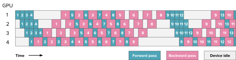
如果仔细计算的话会发现气泡的大小仍然相同,因此训练效率并未显著提升。然而,我们仅需存储 $p$ 个微批次的激活(其中 $p$ 为流水线并行度),而不是 $m$(其中 $m$ 是微批次数量)。这主要是因为观察最后一个阶段的GPU4,如果要做到1f1b的调度,那么在微批次1的梯度返回给第一个GPU的时候,第 $p=4$ 个微批次的激活就应该已经到达了GPU4,所以在此之前对于GPU1必然已经计算完了前$p=4$ 个微批次的激活。这减少了在 AFAB 调度中遇到的激活内存爆炸问题。因此,我们可以增加更多微批次,从而实际减少气泡的影响。
这种设置的主要复杂性(如上图所示)在于前向和反向传播不再是完全顺序执行的,各个GPU执行是并行交错执行的,每个GPU有自己调度的节奏,而不再能用同一套代码来统一控制了。这也是流水线并行通常需要对训练代码和建模代码进行大幅修改的原因之一。
代码分析
1. bidirectional_pipeline_communicate
该函数的作用是 处理一个流水线阶段同时向其邻居阶段发送数据和从该邻居阶段接收数据的双向通信 。
支持两种操作:
处理边界条件,如果是第一层就不需要执行send_bwd_recv_fwd,如果是最后一层就不需要执行send_fwd_recv_bwd
确定通信的对象,如果是send_fwd_recv_bwd,那么对象就是下一个流水线的GPU,不然就是上一个
创建一个空的张量用于接收数据
设置并启动同时进行的异步发送和异步接收操作
两个 P2POp 对象:一个用于发送,一个用于接收。异步执行
等待两个异步执行操作结束
返回接收到的数据
1
2
3
4
5
6
7
8
9
10
11
12
13
14
15
16
17
18
19
20
21
22
23
24
25
26
27
28
29
30
31
32
33
34
35
36
37
38
39
40
41
42
43
44
45
46
47
48
49
50
51
52
53
54
55
56
57
58
59
60
61
62
63
64
65
|
def bidirectional_pipeline_communicate(operation, send_tensor, recv_shapes, device, dtype):
"""
处理流水线阶段之间的双向通信,允许同时进行发送和接收操作。
Args:
operation (str): 双向操作的类型 ('send_fwd_recv_bwd' 或 'send_bwd_recv_fwd')
send_tensor: 要发送的张量
recv_shapes: 要接收的张量的形状规格
device: 张量操作的目标设备
dtype: 张量的数据类型
Returns:
torch.Tensor or None: 接收到的张量,如果在流水线的终端阶段则为 None
"""
global STEP
global VERBOSE
is_fwd = (operation == 'send_fwd_recv_bwd')
if (is_fwd and pgm.process_group_manager.pp_is_last_stage) or \
(not is_fwd and pgm.process_group_manager.pp_is_first_stage):
return None
peer_rank = pgm.process_group_manager.pp_next_rank if is_fwd else pgm.process_group_manager.pp_prev_rank
recv_tensor = torch.empty(recv_shapes, requires_grad=True, device=device, dtype=dtype)
reqs = dist.batch_isend_irecv([
dist.P2POp(dist.isend, send_tensor, peer_rank),
dist.P2POp(dist.irecv, recv_tensor, peer_rank)
])
if VERBOSE:
print(f"{operation} | sending {'next' if is_fwd else 'prev'} "
f"{pgm.process_group_manager.pp_rank} -> {peer_rank} | "
f"receiving {'next' if is_fwd else 'prev'} {peer_rank} -> "
f"{pgm.process_group_manager.pp_rank} | STEP {STEP=} | "
f"RANK:{pgm.process_group_manager.pp_rank}", flush=True)
[req.wait() for req in reqs]
torch.cuda.synchronize()
if VERBOSE: STEP += 1
return recv_tensor
|
2. train_step_pipeline_1f1b
该函数实现了1f1b的调度策略,其旨在通过让每个流水线阶段(GPU)在稳定期同时处理一个微批次(micro-batch)的前向传播和另一个微批次的反向传播,并重叠计算与通信,来提高 GPU 的利用率并减少流水线“气泡”(即 GPU 空闲时间)。
整个函数可以分为三个主要阶段:
预热(Warmup)阶段 :用前向传播任务填充流水线。
稳定(Steady State)阶段 :核心的 1F1B 操作,每个阶段同时执行一个前向和一个反向传播。
冷却(Cooldown)阶段 :清空流水线中剩余的反向传播任务。
初始化阶段:
我们假设如上图所示,GPU数量为4,pp_world_size为4,grad_acc_steps=8。
计算预热阶段的微批次的数量:** **num_warmup_microbatches = min(pgm.process_group_manager.pp_world_size - pgm.process_group_manager.pp_rank - 1, data_loader.grad_acc_steps)。如果pp_rank是0,那么其对应的num_warmup_microbatches为3,如果pp_rank是3,那么对应的num_warmup_microbatches为0。
计算在预热阶段之后,需要在稳定状态下处理的微批次数:num_microbatches_remaining = data_loader.grad_acc_steps - num_warmup_microbatches。
判断是否需要数据并行, 如果需要就标记requires_grad_sync=true。
预热阶段:
预热阶段整体与Afab中的实现前向传播类似。
会执行num_warmup_microbatches次下面的操作来进行预热:
通过recv_forward操作获取前一个阶段的input,注意对于第一阶段的pipeline,这会直接返回none,对于其他阶段会进行阻塞等待。
执行自定义的_forward_step函数,得倒output
通过data_loader获取下一个batch
将input作为batch[“hidden_states”]
执行PipelineParallel的forward
如果是pipeline的最后一个阶段还需要计算loss并将loss作为output_tensor
通过send_forward操作来发送输出
将input和output添加到数组中
如果num_microbatches_remaining>0,即稳定状态下需要微批次那么就再执行recv_forward操作来收集input,这是作为稳定状态循环的开始,一般都需要
如果启用了数据并行,那么还需要先设置require_backward_grad_sync为false,防止还没都最后一个梯度计算就开始执行了梯度平均。
稳定阶段:
在稳定阶段,每个GPU同时执行一个前向传播和反向传播
执行刚刚最后收集到的input的前向传播_forward_step
执行send_fwd_recv_bwd操作发送前向传播的结果收集反向传播的梯度
将当前的input和output都放入到数组中
此时数组中的第一个input和第一个output是一对,直接取出
如果是在最后一个流水线阶段并且是稳定状态的最后一次迭代,那么就说明所有的微批次的反向传播在最后一个阶段都计算完了,设置require_backward_grad_sync为true
执行model.backward来计算反向传播
如果是流水线的最后一个阶段就执行send_backward发送回梯度,不然就执行send_bwd_recv_fwd,发送梯度,等待下一轮的激活值
冷却阶段:
在冷却阶段需要把还剩余的梯度处理掉,因为之前预热阶段对num_warmup_microbatches批次只处理了前向传播,没有处理反向传播,所以这里需要把之前欠缺的反向传播补足。它会遍历需要的反向传播的次数:
如果是最后一次迭代,就设置require_backward_grad_sync=true,使得该批次的梯度可以得到平均
从数组中弹出input和output
调用recv_backward来接收上一个阶段的梯度
反向传播计算梯度
将计算得到梯度通过调用send_backward来将梯度传给前一个阶段
1
2
3
4
5
6
7
8
9
10
11
12
13
14
15
16
17
18
19
20
21
22
23
24
25
26
27
28
29
30
31
32
33
34
35
36
37
38
39
40
41
42
43
44
45
46
47
48
49
50
51
52
53
54
55
56
57
58
59
60
61
62
63
64
65
66
67
68
69
70
71
72
73
74
75
76
77
78
79
80
81
82
83
84
85
86
87
88
89
90
91
92
93
94
95
96
97
98
99
100
101
102
103
104
105
106
107
108
109
110
111
112
113
114
115
116
117
118
119
| def train_step_pipeline_1f1b(model, data_loader, tensor_shapes, device, dtype):
num_warmup_microbatches = min(pgm.process_group_manager.pp_world_size - pgm.process_group_manager.pp_rank - 1, data_loader.grad_acc_steps)
num_microbatches_remaining = data_loader.grad_acc_steps - num_warmup_microbatches
logging_loss, input_tensors, output_tensors = 0.0, [], []
requires_grad_sync = pgm.process_group_manager.dp_world_size > 1
def _forward_step(input_tensor):
batch = next(data_loader)
batch["hidden_states"] = input_tensor.to(device) if input_tensor is not None else input_tensor
output_tensor = model.forward(input_ids=batch["input_ids"].to(device), position_ids=batch["position_ids"].to(device), hidden_states=batch["hidden_states"])
if pgm.process_group_manager.pp_is_last_stage:
output_tensor = F.cross_entropy(output_tensor.transpose(1, 2), batch["target_ids"].to(device), reduction='mean')
nonlocal logging_loss
logging_loss += output_tensor.item() / data_loader.grad_acc_steps
return output_tensor
for _ in range(num_warmup_microbatches):
input_tensor = pipeline_communicate(operation='recv_forward', shapes=tensor_shapes, device=device, dtype=dtype)
output_tensor = _forward_step(input_tensor)
pipeline_communicate(operation='send_forward', tensor=output_tensor, device=device, dtype=dtype)
input_tensors.append(input_tensor)
output_tensors.append(output_tensor)
if num_microbatches_remaining > 0:
input_tensor = pipeline_communicate(operation='recv_forward', shapes=tensor_shapes, device=device, dtype=dtype)
if requires_grad_sync:
model.require_backward_grad_sync = False
for ith_microbatch in range(num_microbatches_remaining):
is_last_iteration = (ith_microbatch == num_microbatches_remaining - 1)
output_tensor = _forward_step(input_tensor)
output_tensor_grad = bidirectional_pipeline_communicate(operation='send_fwd_recv_bwd', send_tensor=output_tensor, recv_shapes=tensor_shapes, device=device, dtype=dtype)
input_tensors.append(input_tensor)
output_tensors.append(output_tensor)
input_tensor, output_tensor = input_tensors.pop(0), output_tensors.pop(0)
if num_warmup_microbatches == 0 and is_last_iteration:
model.require_backward_grad_sync = True
input_tensor_grad = model.backward(input_tensor, output_tensor, output_tensor_grad)
if is_last_iteration:
input_tensor = None
pipeline_communicate(operation='send_backward', tensor=input_tensor_grad, device=device, dtype=dtype)
else:
input_tensor = bidirectional_pipeline_communicate(operation='send_bwd_recv_fwd', send_tensor=input_tensor_grad, recv_shapes=tensor_shapes, device=device, dtype=dtype)
for ith_warmup_microbatches in range(num_warmup_microbatches):
if requires_grad_sync:
model.require_backward_grad_sync = (ith_warmup_microbatches == num_warmup_microbatches - 1)
input_tensor, output_tensor = input_tensors.pop(0), output_tensors.pop(0)
output_tensor_grad = pipeline_communicate(operation='recv_backward', shapes=tensor_shapes, device=device, dtype=dtype)
input_tensor_grad = model.backward(input_tensor, output_tensor, output_tensor_grad)
pipeline_communicate(operation='send_backward', tensor=input_tensor_grad, device=device, dtype=dtype)
return logging_loss
|